FEATool has been designed to be able to perform MATLAB multiphysics simulations in all spatial dimensions (1D, 2D, and 3D). However, running full 3D simulations often requires a significant amount of computational resources, that is memory and simulation time. It is therefore desirable to find simplifications to reduce simulations to two or even one dimension if possible. This post looks at how to transform and modify standard Cartesian PDE equations to axisymmetric form. (Although these examples uses the custom equation approach to set up and run the model, the FEATool GUI with predefined axisymmetric physics modes can be used as well.)
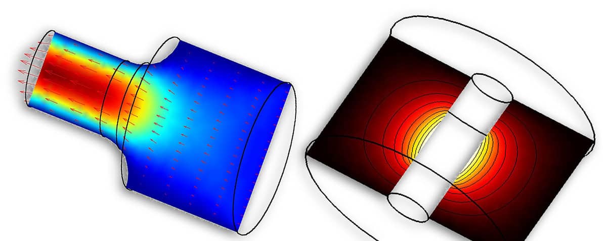
Problems which feature cylindrical and rotationally symmetric geometries and solutions can be reduced to 2D through an axisymmetric coordinate transformation (sometimes also referred to as 2.5D). A symmetry axis, usually r = 0, is taken as reference around which the coordinates, gradient, and divergence operators are transformed. In this way the governing equations will be reduced to two dimensions while featuring a rotationally symmetric three dimensional solution.
All FEATool physics modes that support axisymmetric formulations come with corresponding pre-defined equations. These are available in the FEATool GUI by choosing the 2D Axi coordinate option in the New tab.
It is also possible to manually modify the existing equations or enter user-defined ones. For example, a typical 2D convection and diffusion equation for the unknown c can in the FEATool PDE equation syntax be rewritten from the Cartesian coordinate form
c' - D*(cx_x + cy_y) + (u*cx_t + v*cy_t) = R
to the following axisymmetric form
r*c' - r*D*(cr_r + cz_z) + r*(u*cr_t + v*cz_t) = r*R
Here D is the diffusion coefficient, u and
v the convection velocities, and R reaction
coefficient. In this case it is sufficient to simply replace
x with r and y with
z, and multiply the whole equation with the
r coordinate. Note that the underscore t for
example in cx_t indicates that the coefficient is
multiplied with a test function and treated implicitly in the finite
element context (the time derivative is indicated with a single quote
as in the first term c') .
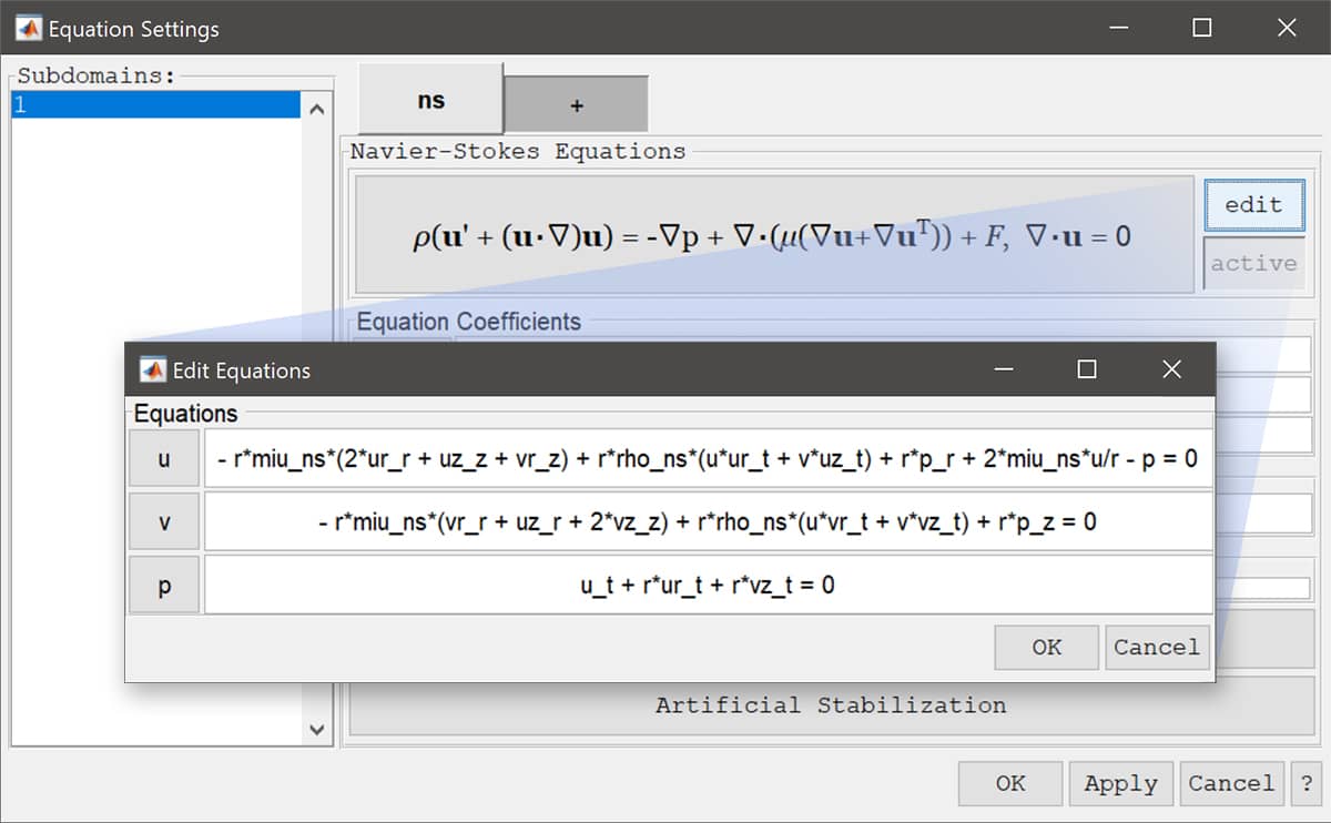
More complex equations are treated analogously, for example the axisymmetric Navier-Stokes equations in the FEATool syntax transform to
-r*miu_ns*(2*ur_r + uz_z +   vr_z) + r*rho_ns*(u*ur_t + v*uz_t) + r*p_r + 2*miu_ns*u/r - p = 0
-r*miu_ns*(  vr_r + uz_r + 2*vz_z) + r*rho_ns*(u*vr_t + v*vz_t) + r*p_z = 0
u_t + r*ur_t + r*vz_t = 0
In addition to modifying the equations an appropriate boundary condition for the symmetry boundary at r = 0 must be chosen such as a homogeneous or symmetry Neumann condition or slip condition for the Navier-Stokes equations.
To perform custom axisymmetric modeling one can either use the custom equation physics mode to define PDEs from scratch, or the edit equation GUI feature by clicking on the edit eqn button in the Equation Settings dialog box. This will show the full equations which can be edited directly as shown in the image below.
Moreover, as usual it is also possible to perform MATLAB script modeling on the command line. A tutorial example modeling axisymmetric fluid flow can be found in the FEATool documentation
In addition, three other axisymmetric model m-script examples can be found in the examples directory of the FEATool distribution.