Different Ways of Working with FEATool and FEM Simulations

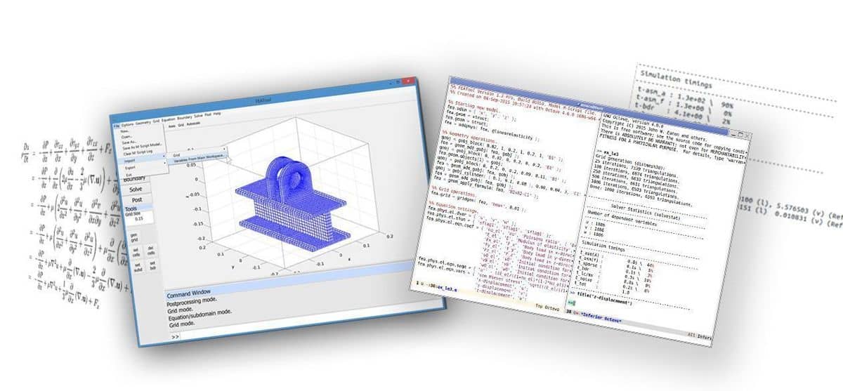
FEATool Multiphysics is unique in that it allows several different ways for users to work with FEM modeling and simulation. The whole spectrum from using the high-level graphical user interface down to low-level access of the fundamental matrices of the underlying finite element FEM discretization is possible. On top of this, since FEATool is written in m-script code, it can be extended and combined with MATLAB toolboxes and custom m-file scripts and functions. This post explains the following four different ways of working with FEATool

1. Graphical User Interface (GUI)

2. Pre-defined physics modes

3. Weak FEM equation formulation

4. Direct matrix assembly

where the last three approaches involve eschewing the GUI for the MATLAB command lines and m-script files.

Graphical User Interface (GUI)

Designed with ease of use in mind, the graphical user interface or GUI is usually the first way one works with FEATool.

Although simple in nature, the FEATool GUI allows for some powerful features that can be utilized to extend code functionality.

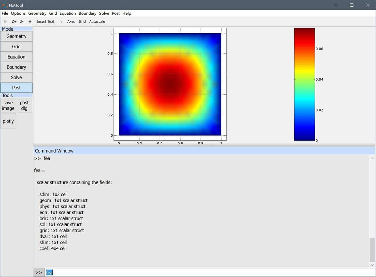
Firstly, in the lower part of the main GUI workspace, right below the Command Window output log, is the FEATool command prompt » which can accept and interpret MATLAB commands. The entered commands are evaluated in the local FEATool memory workspace and thus allows using MATLAB operations without exporting models to the main MATLAB workspace. The variable fea contains the FEATool finite element struct for the current model. For example, try entering the command

fea

to see what the fea struct contains. More information about the composition of the fea struct can be found in the FEATool User’s Guide. Be aware that manipulating this variable directly in the GUI may cause the program to crash if invalid input is given.

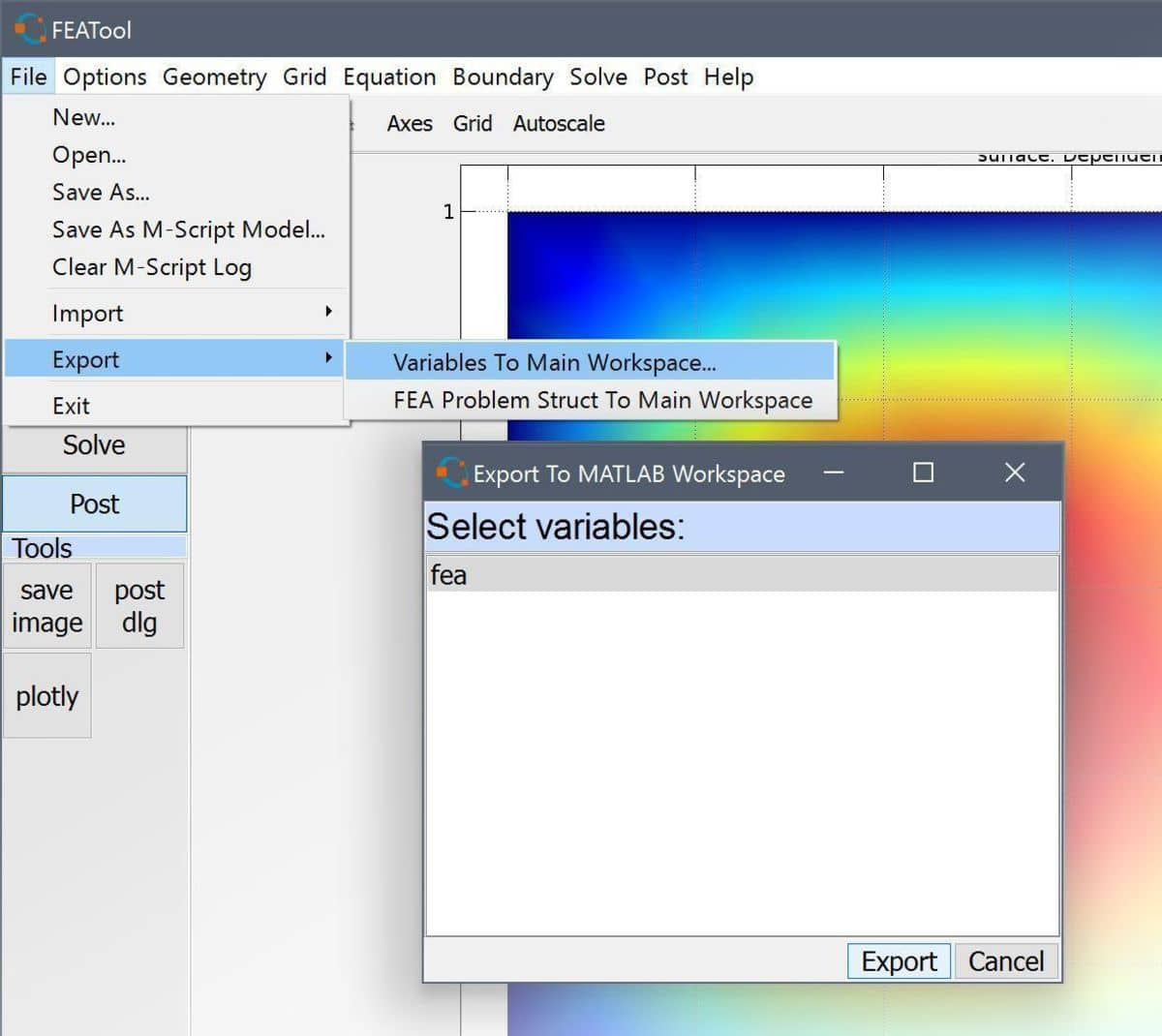
Furthermore, it is possible to import and export data and variables between the GUI and MATLAB main command line workspaces by using the corresponding Import and Export menu options under the File menu.

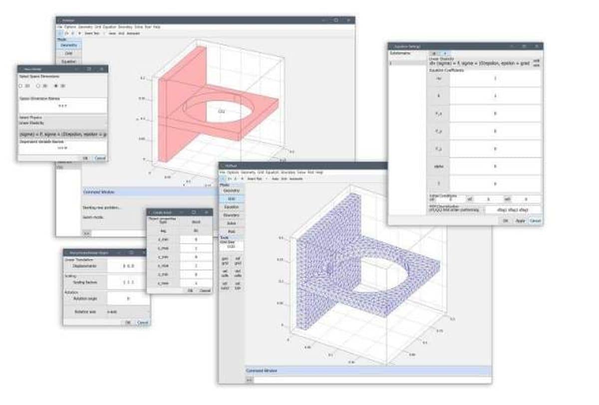
Pre-defined physics modes

The first step in working with MATLAB command line and m-script FEATool models is generally to use the pre-defined physics modes. A good way to understand and learn how FEATool script models are built up and constructed is to use the Save As M-Script Model… option instead of the binary .fea format file.

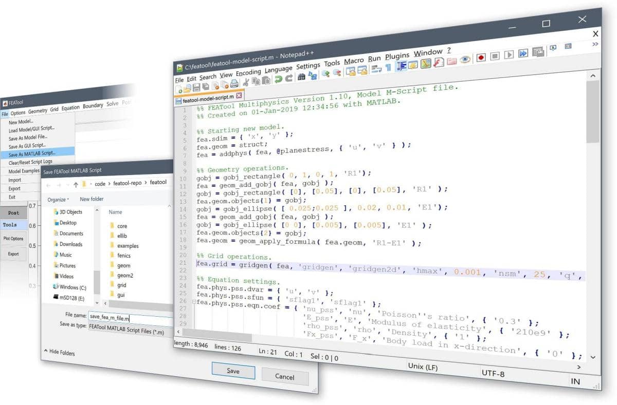
The output .m model source files can be opened in any text editor and the shown output corresponds directly with how the model was constructed in the GUI. Everything from the geometry definition, to solving and postprocessing has corresponding MATLAB function commands.

An example of solving the Poisson equation for a unit circle defined with the Poisson physics mode can be found in the tutorial section of the FEATool documentation As can be seen in the example code, the physics modes are stored in the fea.phys field of the fea model definition struct. The actual strong PDE formulation is defined in the seqn sub-field, in this case

fea = addphys( fea, @poisson );
fea.phys.poi.eqn.seqn = 'dts_poi*u' - d_poi*(ux_x + uy_y) = f_poi'

PDE equation coefficients can be specified as

fea.phys.poi.eqn.coef = { 'dts_poi' [] [] { 1 } ;
                          'd_poi'   [] [] { 1 } ;
                          'f_poi'   [] [] { 1 } ;
                          'u0_poi'  [] [] { 0 } };

where u0_poi is the initial condition for the dependent variable u as defined in fea.phys.poi.dvar. Similarly Dirichlet and Neumann boundary conditions can be prescribed through the bcr_poi and bcg_poi coefficients, respectively

fea.phys.poi.bdr.sel  = 1;
fea.phys.poi.bdr.coef = ...
 { 'bcr_poi' [] [] [] [] [] { 0 } ;
   'bcg_poi' [] [] [] [] [] { 1 } };

Lastly, the command parsephys

fea = parsephys( fea );

parses the equations in all the fea.phys structs and enters the corresponding weak finite element formulations into the global fea.eqn and fea.bdr multiphysics fields.

Weak FEM equation formulation

If one prefers to directly work with the FEM weak formulations this is also possible as shown here for the same Poisson problem as above. Note how there is no phys field or call to parsephys necessary when directly prescribing the fea.eqn and fea.bdr fields

fea.eqn.a.form = { [2 3; 2 3] };
fea.eqn.a.coef = { [1 1] };
fea.eqn.f.form = { 1 };
fea.eqn.f.coef = { 1 };

n_bdr          = max(fea.grid.b(3,:));
fea.bdr.d      = cell(1,n_bdr);
[fea.bdr.d{:}] = deal(0);
fea.bdr.n      = cell(1,n_bdr);

Direct matrix assembly

Finally, for advanced FEM users it is entirely possible to use the core finite element assembly routines assemblea and assemblef to assemble the system matrix and right hand side/load vector after which they can be directly manipulated. Again, the corresponding Poisson problem example is described in the CLI Poisson equation tutorials. The source code for the matrix and source term vector assembly looks like the following

form  = [2 3;2 3];
sfun  = {'sflag1';'sflag1'};
coef  = [1 1];
i_cub = 3;   % Numerical quadrature rule to use.

[vRowInds,vColInds,vAvals,n_rows,n_cols] = ...
     assemblea( form, sfun, coef, i_cub,  ...
       fea.grid.p, fea.grid.c, fea.grid.a );

A = sparse( vRowInds, vColInds, vAvals, n_rows, n_cols );


form  = [1];
sfun  = {'sflag1'};
coef  = [1];
i_cub = 3;

f = assemblef( form, sfun, coef, i_cub, ...
      fea.grid.p, fea.grid.c, fea.grid.a );

Note that here we have to directly prescribe boundary conditions to the system matrix and right hand side vector.

Altogether one can see that FEATool together with MATLAB allows for many possibilities to set up, perform, and analyze multiphysics FEM simulations.