Supersonic Turbulent Flow Past a Prism

This tutorial example sets up and solves supersonic compressible flow around a triangular prism, with viscous effects and turbulence using the OpenFOAM solver.

The inflow is supersonic at 650 m/s causing shock waves to form when the flow field impacts the prism, and also secondary waves following the trailing edges and wake.

Tutorial

This model is available as an automated tutorial by selecting Model Examples and Tutorials... > Fluid Dynamics > Supersonic Turbulent Flow Past a Prism from the File menu. Or alternatively, follow the step-by-step instructions below.

1. To start a new model click the New Model toolbar button, or select New Model... from the File menu.
2. Select the Compressible Flow physics mode from the Select Physics drop-down menu.

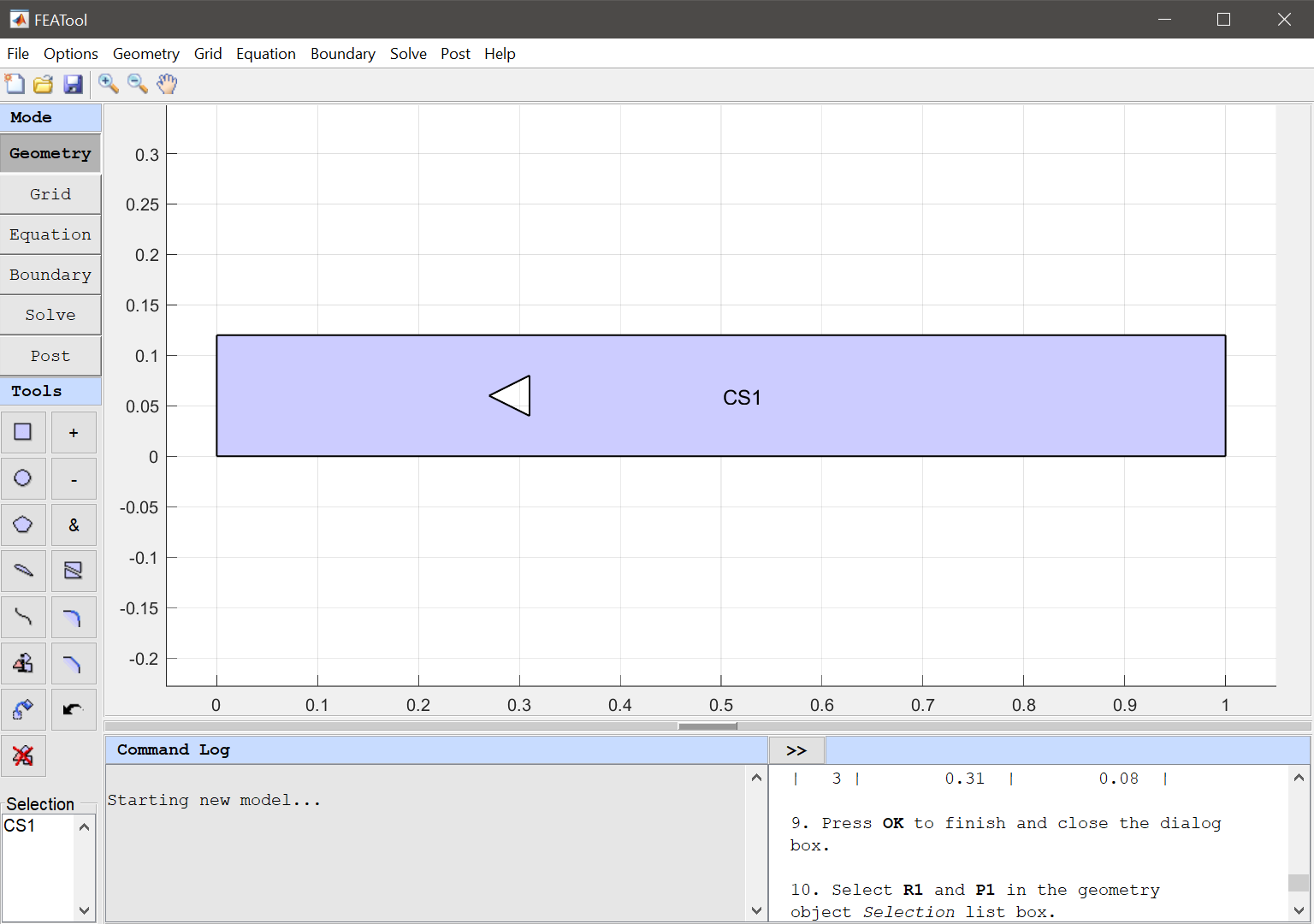
The geometry can be created by subtracting a triangle from a 1 by 0.12 m rectangle.

1. Press OK to finish the physics mode selection.
2. Select Rectangle from the Geometry menu.
3. Enter 1 into the x_max edit field.
4. Enter 0.12 into the y_max edit field.
5. Press OK to finish and close the dialog box.
6. Select Polygon from the Geometry menu.

Enter the following data into the Point coordinates table.

	x	y
1	0.27	0.06
2	0.31	0.04
3	0.31	0.08

1. Press OK to finish and close the dialog box.
2. Select R1 and P1 in the geometry object Selection list box.

3. Press the - / Subtract geometry objects Toolbar button.

   
4. Switch to Grid mode by clicking on the corresponding Mode Toolbar button.

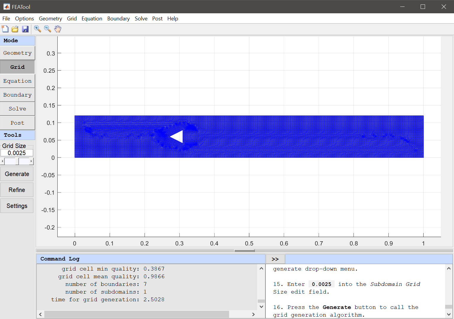
Create a mesh of quadrilateral grid cells, which are better suited for these flow problems.

1. Press the Settings Toolbar button.
2. Select Quad from the Grid cell type to generate drop-down menu.
3. Enter 0.0025 into the Subdomain Grid Size edit field.
4. Press the Generate button to call the grid generation algorithm.

5. Press OK to finish and close the dialog box.

   
6. Switch to equation mode and enter the following fluid parameters, and placeholder coefficient names for the initial conditions.
7. Enter 28.9 into the Molecular weight edit field.
8. Enter 1005 into the Heat capacity at constant pressure edit field.
9. Enter 0 into the Heat of fusion edit field.
10. Enter T0 into the Initial condition for T edit field.
11. Enter u0 into the Initial condition for u edit field.
12. Enter v0 into the Initial condition for v edit field.
13. Enter p0 into the Initial condition for p edit field.

14. Press OK to finish the equation and subdomain settings specification.

    
15. Press the Constants Toolbar button, or select the corresponding entry from the Equation menu, to open the Model Constants and Expressions dialog box. Enter the following constants for the fluid parameters.

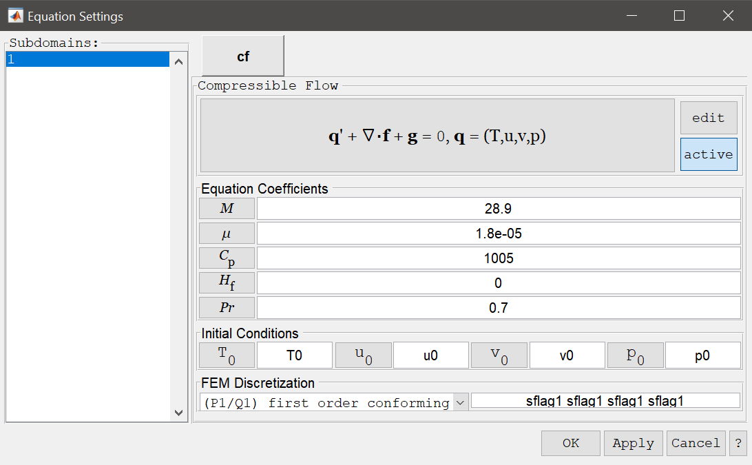
Name	Expression
T0	300
u0	650
v0	0
p0	100000

1. Switch to Boundary mode by clicking on the corresponding Mode Toolbar button.

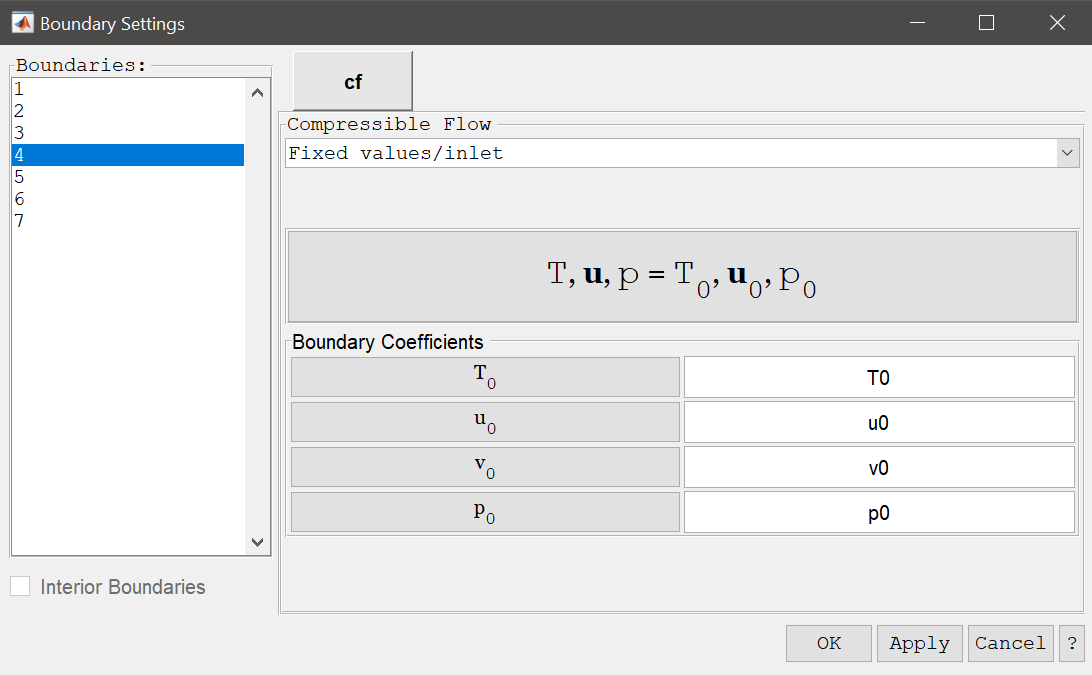
Prescribe the pre-defined constants on the left inlet boundary.

1. Select 4 in the Boundaries list box.
2. Select Fixed values/inlet from the Compressible Flow drop-down menu.
3. Enter T0 into the temperature edit field.
4. Enter u0 into the x-velocity edit field.
5. Enter v0 into the y-velocity edit field.

6. Enter p0 into the pressure edit field.

   

Select Free stream/slip conditions for the top and bottom boundaries.

1. Select 1 and 3 in the Boundaries list box.
2. Select Free stream/slip from the Compressible Flow drop-down menu.
3. Enter T0 into the temperature edit field.
4. Enter u0 into the x-velocity edit field.
5. Enter v0 into the y-velocity edit field.
6. Enter p0 into the pressure edit field.

Set the right outlet boundary to Outlet/inlet boundary (which allows for flow back into the domain if required).

1. Select 2 in the Boundaries list box.
2. Select Outlet/inlet boundary from the Compressible Flow drop-down menu.
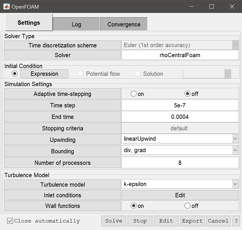
3. Enter T0 into the temperature edit field.
4. Enter u0 into the x-velocity edit field.
5. Enter v0 into the y-velocity edit field.
6. Enter p0 into the pressure edit field.
7. Press OK to finish the boundary condition specification.
8. Switch to Solve mode by clicking on the corresponding Mode Toolbar button.

It is required to use the OpenFOAM CFD solver to solver compressible viscous flow.

1. Press the OpenFOAM Toolbar button.
2. Select the off radio button.
3. Enter 5e-7 into the Time step size edit field.
4. Enter 0.0004 into the Simulation end time edit field.

Select the k-epsilon turbulence model to account for turbulent effects.

1. Select k-epsilon from the Turbulence model drop-down menu.
2. Press the Edit button.
3. Enter 1000 into the Turbulent kinetic energy edit field.
4. Enter 266000 into the Turbulent dissipation rate edit field.
5. Press OK to finish and close the dialog box.

6. Press the Solve button.

   
   

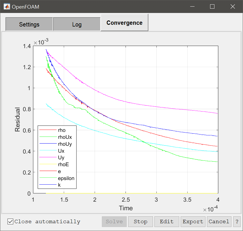
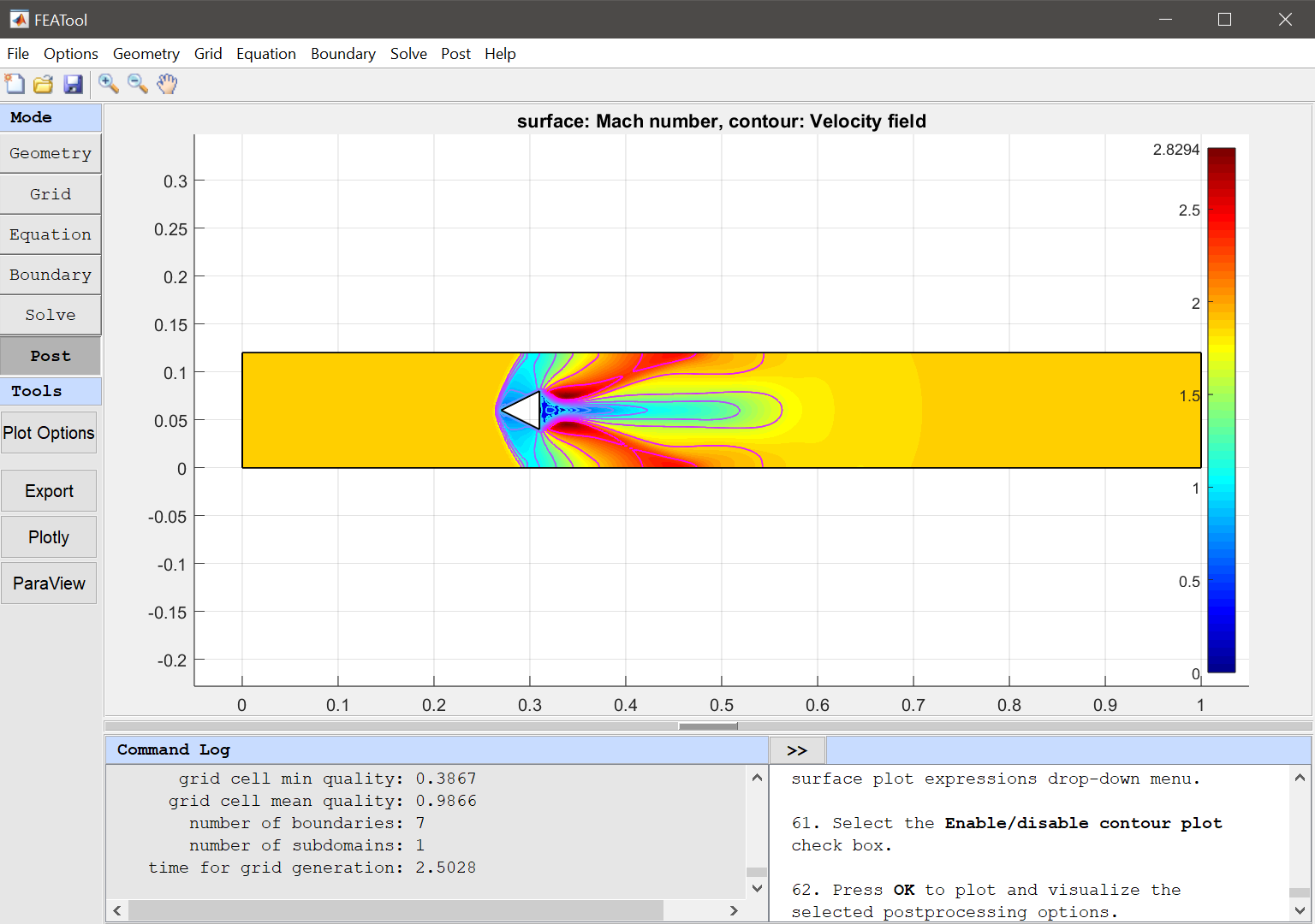
After the problem has been solved FEATool will automatically switch to postprocessing mode, and display the computed velocity field. To change the plot, open the postprocessing settings dialog box by clicking on the Plot Options Toolbar button and plot the Mach number (Ma).

1. Press the Plot Options Toolbar button.
2. Select Mach number from the Predefined surface plot expressions drop-down menu.
3. Select the Enable/disable contour plot check box.

4. Press OK to plot and visualize the selected postprocessing options.

   

Verify that shock waves are formed in front of the prism with some smaller shocks followin the trailing edges.

The supersonic flow past a prism fluid dynamics model has now been completed and can be saved as a binary (.fea) model file, or exported as a programmable MATLAB m-script text file, or GUI script (.fes) file.