Custom Equations and the Weak PDE Formulation Equation Syntax

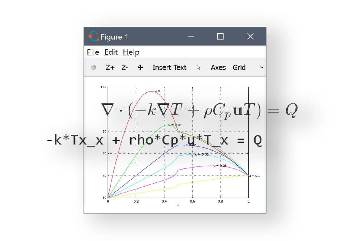
The following post further examines PDE equation parsing and specifying custom equations in FEATool. Furthermore, a simple parametric heat transfer model will be shown and set up as a custom PDE equation, suitable for both the MATLAB command line and m-script file modeling.

Stationary heat transfer by conduction and convection is modeled by the following PDE

\[ \nabla\cdot(-k\nabla T + \rho C_p\mathbf{u}T) = Q \]

where $\rho$ is the density, $C_p$ the heat capacity, $k$ is the thermal conductivity, $Q$ heat source term, and $\mathbf{u}$ a vector valued convective velocity field.

In the FEATool custom PDE equation syntax this equation can in one dimension be written as

-k*Tx_x + rho*Cp*u*T_x = Q

Note that each term may only contain one underscore to indicate that it is a bilinear form to be assembled, meaning that the term is multiplied with a test function to which partial integration is applied as in the usual finite element formulation. The term will then contribute to the implicit FEM system and stiffness matrix. In contrast, this equation looks almost identical

-k*Tx_x + rho*Cp*u*Tx = Q

however, the convective 2nd term, does not feature an underscore and will thus be assembled as a linear term contribution to the right hand side (the force and load vector). The following equivalent equation will thus be solved instead

-k*Tx_x = Q - rho*Cp*u*Tx

If the velocity field is constant or divergence free, these two conservative and non-conservative approaches both lead to the same identical solution, although the latter approach will require a non-linear solver since the right hand side depends on the unknown solution Tx, in this case the first derivative. Also the natural flux (Neumann) boundary conditions will look a little different since they arise from partial integration of the bilinear terms (with the underscores).

To see exactly what resulting weak form contributions results from a custom equation one can use the parseeqn function in the MATLAB workspace. For example

eqn = parseeqn( '-k*Tx_x + rho*Cp*u*T_x = Q' , {'T'}, {'x'} )

will result in the following fields (ignoring eqn.m which specifies the mass matrix for time dependent problems)

>> eqn.a.form{:}

     2      1
     2      2

>> eqn.a.coef{:}

     'k'    '-rho*Cp*u'

The first row in the form equation field specifies trial functions to use for the terms (1=function value, 2=x-derivative, 3=y-derivative, 4=z-derivative), and the bottom row the test functions. Thus in eqn.a a bilinear form is specified which here contains two terms the first $T_x\cdot v_x$ with coefficient k, where $v$ is the finite element test function, and the second $T\cdot v_x$ with coefficient -rhoCpu. Similarly, inspecting the right hand side f field, we have

>> eqn.f.form{:}

     1

>> eqn.f.coef{:}

    'Q'

Compare that with the second non-conservative PDE formulation which instead will result in one term for the bilinear form in eqn.a but two linear forms in eqn.f

Let’s build a simple heat transfer model with the FEM weak form. First we define a finite element ‘fea’ struct and name the 1D space dimension to x, we also need a grid, in this case a line from 0 to 1 with 100 grid cells

fea.sdim = { 'x' };
fea.grid = linegrid( 100, 0, 1 );

Furthermore, we name out dependent variable or unknown to T for temperature and use 1st order linear Lagrange FEM shape functions to approximate the solution

fea.dvar = { 'T' };
fea.sfun = { 'sflag1' };

Now we define the equations in the fea.eqn field as described above. The equation coefficient and expressions are specified in a cell array in the fea.coef or fea.expr fields

fea.eqn  = parseeqn( '-k*Tx_x + rho*Cp*u*T_x = Q', ...
                     fea.dvar, fea.sdim );
fea.coef = { 'k',    '1e-3 + 0.01*(x>0.5)' ;
             'rho',   1 ;
             'Cp'     1 ;
             'u'      0 ;
             'Q'      1 };

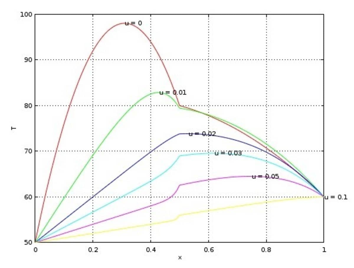
Note, that to make it more interesting we have defined a discontinuous thermal conductivity k = 1e-3 + 0.01*(x>0.5) that will take on the value 1e-3 in the first half of the domain (x<0.5) and 1e-3 + 0.01 = 0.011 in the second half.

Fixed value (Dirichlet) and flux (Neumann) boundary conditions are defined in the fea.bdr.d and fea.bdr.n fields, respectively. In this case we fix the temperature to 50 and 60 degrees at the two end points.

fea.bdr.d = { 50 60 };
fea.bdr.n = { [] [] };

Finally, the following small script solves and plots the solution for a number of different velocity u values.

figure, hold on
uvals  = { '0' '0.01' '0.02' '0.03' '0.05' '0.1' };
colors = { 'r' 'g'    'b'    'c'    'm'    'y'   };
for i=1:numel(uvals)

  fea.coef{4,2} = uvals{i};
  fea = parseprob( fea );
  fea.sol.u = solvestat( fea );

  postplot( fea, 'surfexpr', 'T', 'color', colors{i} )

  [umax,j] = max( fea.sol.u );
  text( fea.grid.p(j), umax, ['u = ',uvals{i}] )
end
ylabel( fea.dvar{1} )
xlabel( fea.sdim{1} )
axis(  [0 1 50 100] )
axis normal
grid on

Resulting in the following parametric solutions for the temperature distribution.