This tutorial illustrates how to couple a heat transfer model with linear elasticity by manually defining the multiphysics equations with the FEATool PDE syntax. The custom model examines how temperature rise in a brake disk under braking results in heat induced displacements with resulting increased stresses and strains. Using the assumption that all variations in the rotational direction can be neglected it is possible to use an axisymmetric formulation in cylindrical coordinates, saving a significant amount of computational time and resources compared to full 3D simulations.
Previous tutorial articles have introduced the axisymmetric equations for stresses and strains as well as heat transfer and general transport equations. The temperature equation for heat conduction in axisymmetric form can simply be defined as
eqn_T = 'r*rho*cpd*T'' - r*K*(Tr_r + Tz_z) = 0';
where rho is the density, cp the heat capacity, K the thermal conductivity, and r and z the space dimension coordinates. (Although this tutorial uses the MATLAB m-script and custom equation approach to set up and run the model, the FEATool GUI with predefined axisymmetric physics modes can be used as well.)
The PDE equations used for calculating the displacements u and w are here reformulated for stability by multiplying the r-equation with r 2 and substituting and solving for u/r instead of just u, and additionally multiplying the z-equation with r. This eliminates divisions by r at the center r = 0 line. Moreover, the equations also here incorporate the temperature strain relation $\epsilon_{th} = \alpha(T-T_{ref})$. The resulting axisymmetric stress-strain equations read
eqn_r = ['- lambda*( c1*r^3*ur_r + r^2*wz_r ) - lambda*c2*( r^3*uz_z + r^2*wr_z  )', ...
         '- lambda/nu*r^2*u_r + lambda/nu*r^2*ur_t + lambda*2*r*wz_t + lambda/nu*2*r*u_t', ...
         '+ r^2*c3*( T - T_ref )_r - 2*r*c3*( T - Tref )_t = 0'];

eqn_z = ['- lambda*c2*( r^2*uz_r + r*wr_r ) - lambda*( r^2*ur_z + c1*r*wz_z )', ...
         '- lambda*2*r*u_z + r*c3*( T - T_ref )_z = 0'];
with the equation coefficients $\lambda = E\frac{\nu}{(1+\nu)(1-2\nu)}$, $c_1 = \frac{1-\nu}{\nu}$, $c_2 = \frac{1-2\nu}{2\nu}$, and $c_3 = \alpha\frac{E}{1-2\nu}$.
When a constant reference temperature T_ref is used implicit bilinear forms involving the temperature T, as well as the weak equation linear right hand side (RHS) source terms $-\int r^2c_3T_{ref}\frac{\partial \phi_u}{\partial r} d\Omega$ and $-\int rc_3T_{ref}\frac{\partial \phi_u}{\partial z} d\Omega$ will automatically be added.
The temperature T is here coupled to the displacements u (here redefined as u/r) and w, that is a one-way multiphysics coupling (as the temperature field is assumed to not depend on the deformation of the disk). The problem is also quasi-static in that the temperature field is time dependent, while the stresses are static (in each time step). The following command statements
fea.sdim = { 'r' 'z' };
fea.dvar = { 'u' 'w' 'T' };
fea.sfun = { 'sflag2' 'sflag2' 'sflag2' };
fea.eqn  = parseeqn( { eqn_r eqn_z eqn_T }, fea.dvar, fea.sdim );
take the FEATool strong PDE equation form above, parses it, and fills out the fea.eqn weak equation struct (that is the eqn.(*). form, coef, and sfun fields).
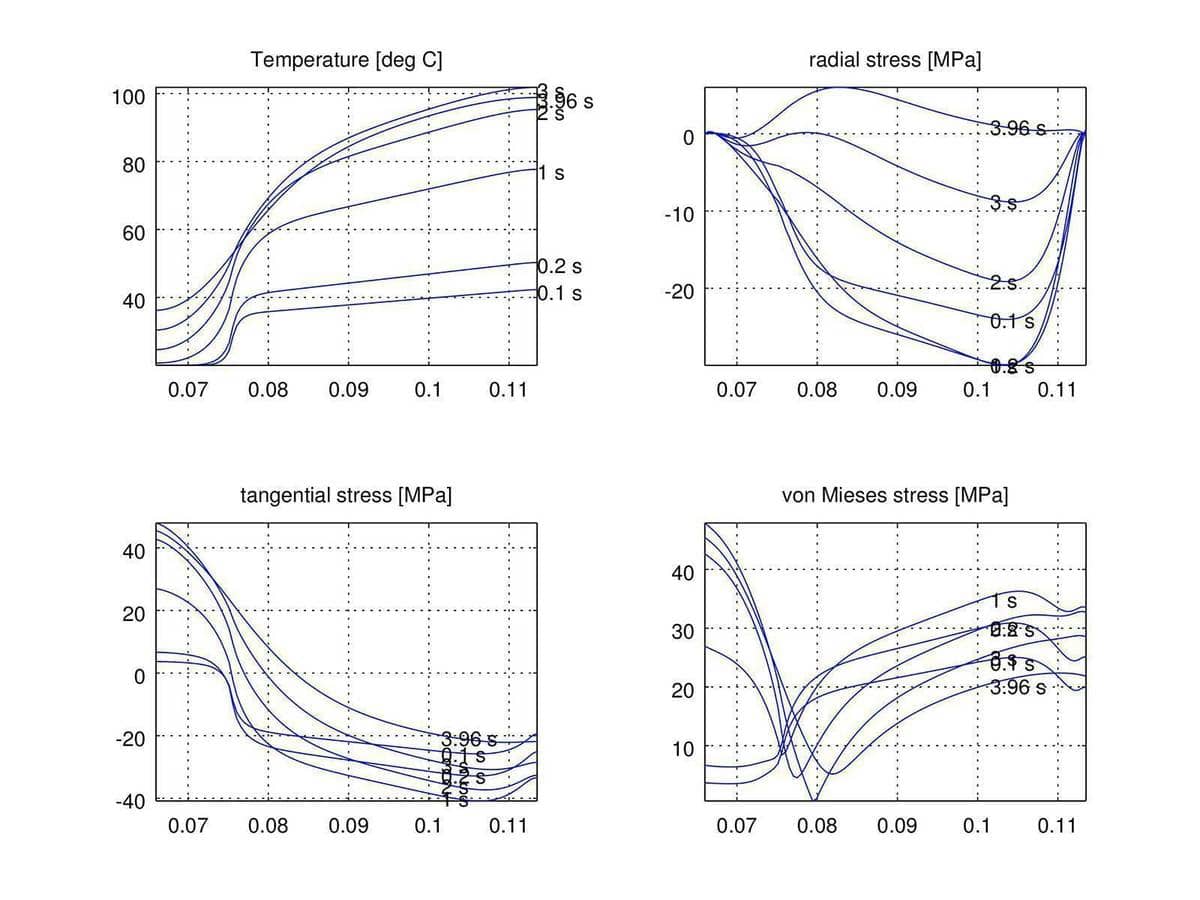
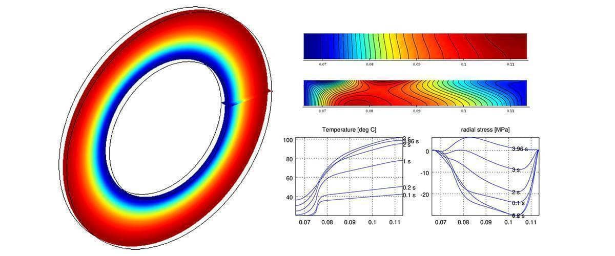
Reference simulations have been performed with the geometry and material parameters given in the paper [1] resulting in the final temperature and stress fields shown in the figure below.

The resulting temperature and stress curves on the disk surface at various times also agree well with the results computed by Nastran FEM solver in reference [1].

The complete custom PDE FEATool brake disk simulation MATLAB m-script model using the pre-defined axisymmetric stress-strain physics mode is available as the ex_axistressstrain4 model in the FEATool examples directory.
[1] A. Adamowicz, Axisymmetric FE Model to Analysis of Thermal Stresses in a Brake Disk, Journal of Theoretical and Applied Mechanics, 53, 2, pp. 357-370, Warsaw 2015.
