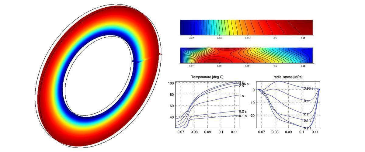
The following post breaks down and explains the postprocessing and visualization steps used to create the images and video for the axisymmetric stress-strain brake disk analysis model. By using the Octave or MATLAB command line and exported finite element fea data struct one can create custom graphics and visualizations that is currently not possible to do within the FEATool graphical user interface (GUI).
The first step in creating the advanced visualizations is to run the
FEATool model example m-script file to generate and return the finite
element analysis struct fea, together with the solution stored in
the fea.sol.u field (in this case the automatic pre-defined plots
can be turned off with the ‘iplot’, ‘0’ flag, since
postprocessing will be done manually)
fea = ex_axistressstrain4( 'iplot', 0 );
Next, model constants and parameters used in during postprocessing are prescribed
deltad = 5.5e-3;     % Disk thickness.
rd     = 66e-3;      % Disk inner radius.
rp     = 75.5e-3;    % Pad inner radius.
Rd     = 113.5e-3;   % Disk outer radius.
Continuing, the solution vector for all time steps is saved in a temporary variable u (the solution at each time step corresponds to a column in u). The parameters cmax and cmin are also calculated which later are used to fix the colormap range (otherwise not much difference between hot and cold maxima can be seen)
u    = fea.sol.u;
cmax = max(u(:)) - 273.15;
cmin = 0;
Coordinates to plot and visualize the contours and boundaries of the brake disk must also be defined (here the assumption is that the disk is centered at the origin with the radial coordinate spanning the x-z plane)
% Points around the circumference.
npth = 72;
th   = linspace( 0, 2*pi, npth );

% Inner coordinates.
x    = rd*cos(th);
z    = rd*sin(th);

% Outer coordinates.
xx   = Rd*cos(th);
zz   = Rd*sin(th);

y    = deltad*ones(size(x));
The ringgrid function is also
used to generate coordinates around the disk in the grid struct
variable g and evaluation points in rz. These will be used to
interpolate the temperature field from axisymmetric coordinates to
three dimensions (the ring grid can be seen and visualized by itself
using the plotgrid( g ) command)
npr  = 25;
g    = ringgrid( npr-1, npth-1, rd, Rd );
r    = sqrt( g.p(1,:).^2 + g.p(2,:).^2 );
rz   = [rd+sqrt(eps) rd+(Rd-rd)/2 Rd-sqrt(eps);deltad/2*[1 1 1]];
Now, the actual plotting is initialized by creating a figure window to draw in, an empty array for the stresses at the three points (inner radius, outer radius, and the mid point), and starting the postprocessing loop
figure
st = zeros(3,1);
for i=1:size(u,2)
The use subplot MATLAB command is used to hold two horizontal images. First is the 3D temperature field, starting with drawing the black outline of the brake disk
  subplot(1,2,1)
  hold on

  plot3(x,  y, z,'k-')
  plot3(x, -y, z,'k-')
  plot3(xx, y,zz,'k-')
  plot3(xx,-y,zz,'k-')
The i:th solution is selected as the only solution in fea.sol.u (since evalexpr per default uses the solution at the last time step), after which the temperature is evaluated along the radius at the disk center line coordinate (z=0).
  fea.sol.u = u(:,i);
  T = evalexpr( 'T-273.15', [r;zeros(size(r))], fea );
Using the assumption that the solution is axisymmetric, one can extrapolate the data all along the brake disk with the help of the annular grid struct g created earlier. The MATLAB patch command is used to plot the x-z temperature field
  h = patch( 'faces',     g.c', ...
             'vertices',  [g.p(1,:)' zeros(size(g.p,2),1) g.p(2,:)'], ...
             'facevertexcdata', T, ...
             'facecolor', 'interp', ...
             'linestyle', 'none' );
Furthermore, the temperature for the original patch in the positive and mirrored (negative) z-directions is also plotted
  postplot( fea, 'surfexpr', 'T-273.15', 'colorbar', 'off' )
  fea.grid.p(2,:) = -fea.grid.p(2,:);
  postplot( fea, 'surfexpr', 'T-273.15', 'colorbar', 'off' )
  fea.grid.p(2,:) = -fea.grid.p(2,:);
Lastly, a title is set, the color map range fixed, and a suitable viewing angle is chosen
  title( 'Temperature' )
  caxis( [cmin cmax] )
  view(3)
  axis off
  axis tight
For the second subplot the idea is to follow the von Mieses stress as
a function of time for the three points prescribed in rz. Just as
for the temperature, the stress can be evaluated with the
evalexpr command
where the stress expression svm has been defined earlier in the
fea.const field of the model fea struct
  subplot(1,2,2)
  hold on
  grid on
  if( i>1 )   % Skip first zero solution
    st = [st evalexpr( '(svm)*1e-6', rz, fea )];
The stress is plotted as a function of time, with additional text and legends added for identification
    plot( tlist(1:i), st(1,:) )
    plot( tlist(1:i), st(2,:) )
    plot( tlist(1:i), st(3,:) )

    text( tlist(i), st(1,end), 'r = rd' )
    text( tlist(i), st(2,end), 'r = (rd+Rd)/2' )
    text( tlist(i), st(3,end), 'r = Rd' )

    axis( [0 tmax 0 max(st(:))] )
  end
  xlabel( 'Time [s]' )
  ylabel( 'von Mieses stress [MPa]' )
Finally, before closing the loop, a drawing update is forced with the drawnow command, and optionally an jpeg image file is written out and saved for later processing
  drawnow
  print( '-r200', '-djpeg', sprintf('img%03i.jpg',i) )
end
After all the MATLAB postprocessing has finished the images can easily be converted to a video with a suitable tool, such as for example ffmpeg with the command
ffmpeg -i img%03d.jpg -c:v libx264 -vf "fps=25, format=yuv420p, crop=1600:1198:0:0" out.mp4
From the generated video one can now clearly see that the temperature is the highest on the outer two-thirds of the disk consistent with where the brake pad is acting. In contrast the maximum stress is achieved at the inner radius r = rd around t = 3.0 s, and is significantly higher than at the two points measured further out on the disk.
