Space-Time Finite Element (FEM) Simulation
FEATool Multiphysics is a very flexible CAE physics and continuum mechanics simulation toolbox, allowing users to customize, easily define, and solve their own systems of partial differential equations (PDE). In the following it is shown how the custom equation feature can be used to transform a low dimensional transient and time dependent heat-transfer problem, to a higher dimensional but stationary equivalent simulation problem, which potentially can save significant computational time and effort.
The original one-dimensional heat transfer problem considers heat conduction in a 1 m rod where the right end is kept fixed at the initial temperature T = 25 degrees, and the left is subject to a constant and uniform outwards heat flux qn = 1, that is
          +----------- L=1 m ----------+ T = 25
        q_n = 1      T(t=0) = 25
which is governed by the following PDE equation
\[ \left\{\begin{aligned} \rho c_p\frac{\partial T}{\partial t} - \frac{\partial}{\partial x}(k\frac{\partial T}{\partial x}) = 0 \\\ T|_{x=1} = 25, \\\ -\hat{n} \cdot k\frac{\partial T}{\partial x}|_{x=0} = q_n = 1, \\\ T(t=0) = 25 \end{aligned}\right. \]
This one-dimensional transient and instationary problem is typically solved by discretizing the time dependent term with a difference formula of the type
\[ \rho c_p \frac{T^{n+1} - T^{n}}{\Delta t} + \theta A(T^{n+1}) = \theta f^{n+1} + (1-\theta)(f^n - A(T^n)) \]
where for example $\theta = 1$ results in the standard backward Euler scheme, and $\theta = 0.5$ the 2nd order Crank-Nicolson scheme, and where $A$ and $f$ represent the discretized system matrix and source term, respectively.
If a problem requires a lot of small time steps $\Delta t$ it can sometimes be more computationally efficient to consider time as a higher order direction in space (at the cost of higher memory consumption). This means that instead of looking at a temporal sequence of 1D problems (or 1D time slices), we can consider the time-dimension as just another (pseudo) space-dimension and solve a stationary higher dimensional problem for all times at once.
The transformed problem domain will now be a rectangle where time flows from y = 0 to y = tmax. The bottom boundary is equivalent to the initial condition, right and left boundaries are identical to the original problem, and the top is an outflow boundary (for time).
The standard equation for convection and conduction in two dimensions reads
\[ -k\ (\frac{\partial^2 T}{\partial x^2} + \color{red}{\frac{\partial^2 T}{\partial y^2}}) + \rho c_p (\color{red}{u \frac{\partial T}{\partial x}} + \color{blue}{v} \frac{\partial T}{\partial y}) = 0 \]
If one compares this equation to the one dimensional one, the thermal diffusion or conduction term in the y-direction as well as the convection in the x-direction is not be present and should therefore be removed (red terms). The temporal term for the time derivative can here be identified as the convective term in the y-direction with unit velocity (which one can think of as time flowing from the bottom to the top). The resulting equation in the FEATool PDE equation syntax will read
-k*Tx_x + rho*cp*1*Ty_t = 0
In this equation syntax (and finite element weak formulation context which is the basis of the underlying discretization used by FEATool) an underscore _xi denotes partial integration with respect to the corresponding space dimension, while a _t postfix denotes multiplication with the FEM test function space. The equivalent weak equation formulation will therefore be
\[ \int_\Omega ( k\ \frac{\partial T}{\partial x}\frac{\partial \phi}{\partial x} + \rho c_p \frac{\partial T}{\partial y} \phi )\ d\Omega + \int_\Gamma -\hat{n}\cdot k\frac{\partial T}{\partial x}\phi\ d\Gamma = 0 \]
where $\phi$ is the chosen finite element test function space.
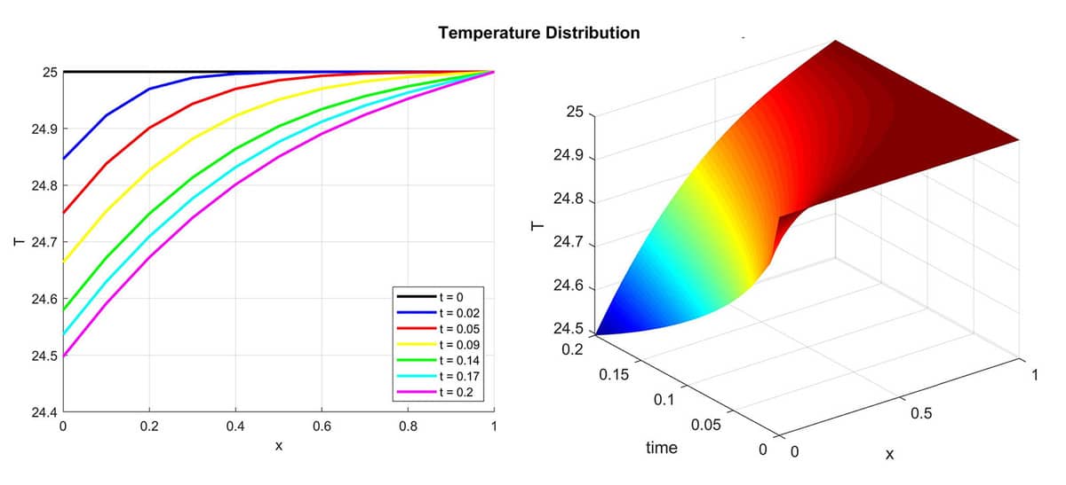
The solution computed with the corresponding 2D space-time transformation is show below (right) and compares very well with the one-dimensional and analytic solutions (left).

Follow the link below for a step-by-step tutorial how to implement this model in the FEATool GUI as well as in the MATLAB m-file scripting language.
Note that the solution the presented problem is very smooth and is therefore very suitable for this technique. If the problem features sharp gradients and/or shocks, then adding artificial stabilization terms might be necessary due to the pure convection type problem in the temporal direction, as it does not feature any built-in stabilizing diffusion.